Better counterfactual componentprediction with submodular quadratic component models

In a previous post, I described a trick for reducing the sample complexity of component attribution using extracted linear models. This post describes a follow-up: we replace the linear component model with a quadratic one, carefully designed so it's still fast to learn and still interpretable. Specifically, by using ideas from Boolean Fourier analysis and submodular optimization, we get better predictions with fewer forward passes, and open the door to more interesting downstream reasoning about groups of components.

The previous post discussed the component attribution problem. There is a large model \(M\) (say a ResNet or a language model) and we want to understand which of its internal components—convolutional filters, attention heads, etc.—matter for a given prediction. The idea behind component attribution (Shah et al., 2024) is to treat this as a prediction problem: learn a lightweight model that predicts what happens when you ablate (zero out) subsets of components.

The method, called COAR (Component Attribution via Regression), works like this:

1. Randomly sample a bunch of ablation masks \(x \in \{0,1\}^n\), where \(x_i = 0\) means component \(i\) is ablated.
2. For each mask, run the model on some test input \(z\) and record the correct-class margin.
3. Fit a linear regression from masks to margins.

The learned coefficients then serve as attribution scores: a large positive coefficient for component \(i\) means ablating it hurts performance, so it's "important." The quality of the fit is measured by the Linear Data Score (LDS), which is the Spearman rank correlation between predicted and actual margins on a held-out set of ablation masks.

This works surprisingly well. But each datapoint requires a full forward pass through a potentially huge model, and you need a separate component model for each test input \(z\). So sample complexity matters a lot.

We could achieve optimal LDS by simply computing ablated forward passes on counterfactuals of interest, so why learn a linear component model? The benefit lies in the way linear models attack a trilemma involving efficiency, interpretability, and usefulness.

• Fast. For large ML models, computing ablated forward passes every time we want to peek at some counterfactual \(x, f(M_z(x))\) is computationally expensive. Thus, we want to estimate \(f(M_z(x))\) given \(x\) using a much more lightweight model, such as a linear model.
• Interpretable. Learning a linear model gives us actual insight into the value of each component, by "reading off" attributions from the coefficients. Due to linearity, the learned coefficient \(\theta_i\) attached to \(x_i\) essentially models the individual contribution of component \(i\) towards increasing correct class margin. This coefficient can thus be used as a proxy for the "importance" of a specific component to a correct prediction of model \(M\) on input \(z\).
• Useful. Linear component models already achieve surprisingly high LDS with reasonable sample size \(m\), and are useful for downstream tasks in model editing (e.g., naive optimization over groups of components).

Linear models are great because they're fast, interpretable, and surprisingly accurate. But there's a natural question: is linearity leaving predictive power on the table?

An obvious change is to use a quadratic model, which would add interaction terms \(x_i x_j\) to capture pairwise effects between components. However, obviosuly, if you have \(n\) components (a ResNet-50 has 22,720 convolutional filters), then a full quadratic model has \(\binom{n}{2}\) interaction terms (approximately 258 million in the case of a ResNet-50). This is far too many parameters, and one would need an absurd number of forward passes to fit it, which defeats the whole purpose.

Can we learn a sparse quadratic model efficiently, without giving up interpretability?

Our proposed approach leans on two ideas from seemingly different areas that turn out to fit together nicely.

Idea 1: Fourier analysis tells us where to look.

A beautiful result from Saunshi et al. (2022) connects component modeling to Boolean harmonic analysis. Any function \(g: \{0,1\}^n \to \mathbb{R}\) has a unique decomposition into Fourier coefficients \(\hat{g}(S)\) indexed by subsets \(S \subseteq [n]\). The degree-1 coefficients \(\hat{g}(\{i\})\) are exactly what linear regression recovers. The degree-2 coefficients \(\hat{g}(\{i,j\})\) capture pairwise interactions.

But which degree-2 coefficients are worth estimating? Here's where a theorem from Feldman and Vondrák (2016) helps. They show that for submodular (or supermodular) functions, the number of large Fourier coefficients on degrees 1 and 2 is bounded. Informally: most interaction terms are negligible. Only the ones involving already-important components tend to matter.

This suggests a simple heuristic: first learn a linear model, identify the top \(k\) components by coefficient magnitude, and then only add interaction terms between those top \(k\) components. Instead of \(\binom{n}{2}\) interactions, you get \(\binom{k}{2}\)—which for \(k = 16\) is just 120 terms.

Idea 2: Encourage supermodularity for better optimization.

The second idea is about what kind of quadratic model to learn. A function is supermodular if ablating component \(i\) hurts more when component \(j\) is also ablated, creating a "compounding damage" property. For degree-2 polynomials, supermodularity corresponds to having nonnegative interaction coefficients.

Why do we care? Because supermodularity (and its dual, submodularity) unlocks powerful optimization algorithms. If we want to find the smallest set of components whose ablation flips a prediction—a natural downstream task—then having a supermodular component model lets us use greedy algorithms with provable approximation guarantees. More on this later.

So during training, we project all negative interaction coefficients to zero at each SGD step. This is a form of inductive bias: it reduces the effective parameter space and encodes a structural assumption about how components interact.

Here's the full pipeline. Steps 1 and 2 are the same as COAR:

1. Sample \(m\) random ablation masks and compute forward passes to get margins. This gives a dataset \(D_z = \{(x^{(i)}, f(M_z(x^{(i)})))\}_{i=1}^{m}\).
2. Fit a linear model \(\theta_{\text{lin}}\) via mini-batch SGD (this is just COAR).
3. Select the top \(k\) components by coefficient magnitude. Let \(K\) be their indices. Augment the model with \(\binom{k}{2}\) interaction terms for all pairs in \(K\).
4. Continue training with projected SGD: at each step, clamp all negative interaction coefficients to zero.

The result is a sparse quadratic model \(\theta_{\text{sq}}\) with \(n + \binom{k}{2}\) parameters, which for \(k \ll n\) is barely larger than the linear model.

We tested this on a ResNet-50 trained on ImageNet (22,720 components). We sampled 50,000 random ablation masks (each component ablated independently with probability 0.1) and evaluated on 16 random test images. LDS was computed on a held-out set of 5,000 ablation masks.

We set \(k = 16\), giving 120 interaction terms. Both COAR and our method were trained for the same number of gradient steps at each sample size: COAR for 300 epochs, our method for 200 epochs linear + 100 epochs quadratic with projected SGD.

Figure 1: Mean LDS vs. sample size for our method compared to COAR, on 16 random ImageNet test images. Shaded regions show 95% confidence intervals via bootstrap. Our method achieves a 20% reduction in the number of forward passes required to achieve LDS around 0.35.

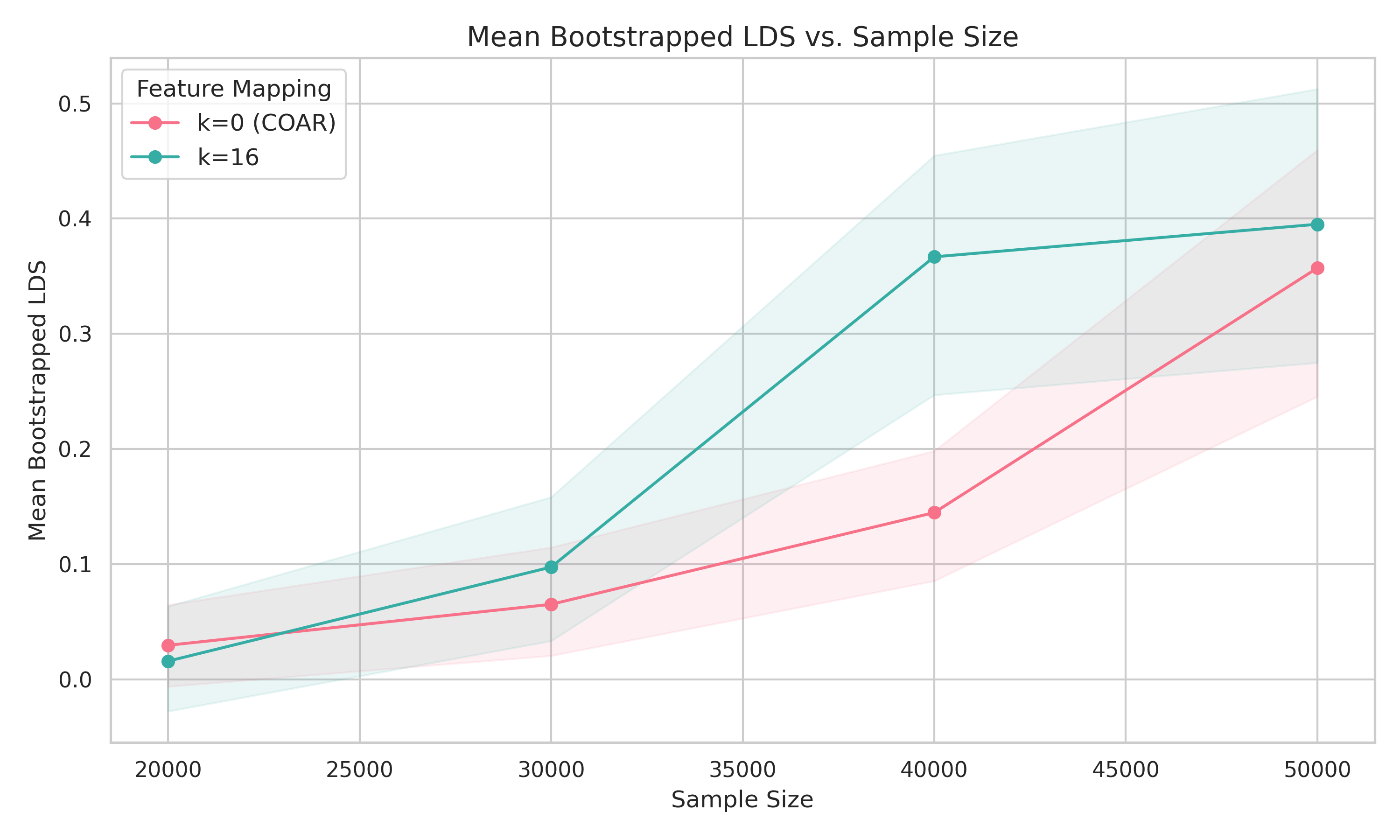
The headline: to achieve LDS around 0.4, our method needs about 40,000 forward passes compared to COAR's 50,000—a 20% reduction. At fixed sample size, we also see a modest but consistent improvement in LDS. The gains are more pronounced at smaller sample sizes, which is exactly where efficiency matters most.

Is 20% earth-shattering? Not on its own. But remember, we're adding only 120 parameters to a model that already has 22,720. The improvement is essentially free in terms of model complexity.

Recall the trilemma. A key property of COAR (a linear model) is that you can "read off" attributions from the linear coefficients. If we use a model with quadratic terms, do we lose that?

The answer is no. It comes from the notion of a discrete derivative in Boolean Fourier analysis. The individual influence of component \(i\) at a point \(x\) is:

This measures how much the function value changes when you toggle component \(i\) on vs. off, scaled by the standard deviation \(\sigma\) of the sampling distribution.

A key fact is that the expected discrete derivative equals the degree-1 Fourier coefficient: \(\mathbb{E}_x[\mathbf{D}_i^p[g(x)]] = \hat{g}(\{i\})\). So COAR's coefficients are really estimating average individual influence. That's useful, but it's an average—it doesn't depend on which other components are currently ablated (i.e., it is not context-aware).

With a quadratic model, we can do better. The discrete derivative has a direct expansion in terms of Fourier coefficients:

Truncating to degree 2, this gives us:

In other words, the individual influence of component \(i\) now depends on the current ablation mask \(x\). If component \(j\) is also ablated, and \(\theta_{ij}\) is large and positive, then the influence of component \(i\) increases. This is what we call a context-aware individual influence estimate, and it strictly generalizes the linear case (which is recovered by averaging over \(x\)).

Suppose you want to answer a question like: what is the smallest set of components that, when ablated, would flip this model's prediction? This is a natural thing to want for debugging, model editing, or understanding fragility.

Formally, we want to solve:

where \(1\) is the "no ablation" mask and \(1 \setminus S\) ablates the components in \(S\).

With a linear model, this is trivial—you just pick the \(k\) components with the largest coefficients. The greedy algorithm collapses to sorting. There's no interaction between choices.

With a supermodular quadratic model, the problem becomes genuinely combinatorial, but in a nice way. Because our model has nonnegative interaction terms, the objective \(\theta(1) - \theta(1 \setminus S)\) is a submodular function of \(S\). And submodular maximization under cardinality constraints is a well-studied problem with good algorithms.

For the monotone case (ablating more components always hurts more), the classic greedy algorithm of Nemhauser et al. (1978) gives a \((1 - 1/e)\)-approximation—about 63% of optimal. And the greedy algorithm here is nontrivially context-aware: at each step, it re-evaluates which component to ablate next, taking into account which components are already ablated, using the context-aware influence formula from above.

For the non-monotone case (where ablations can sometimes help), there are algorithms like that of Buchbinder and Feldman (2018) that give a \(1/e\)-approximation in \(O(k^3 n)\) time.

None of this is possible with a purely linear component model. The quadratic structure is what makes the optimization nontrivial and the greedy algorithm meaningful.

In the previous post, I described a different trick: train a 2-layer ReLU network and then extract a linear model by removing the ReLU activations and multiplying the weight matrices together. That approach also reduces sample complexity (by 40-60% on smaller models), but for different reasons—it leverages the implicit bias of neural network training.

The quadratic approach here is more principled: we have a clear theoretical story (Fourier analysis, submodularity) for why it works and what the coefficients mean. The two ideas aren't mutually exclusive—you could imagine combining them—but the quadratic approach has the advantage of opening up the optimization applications via submodularity.

The main takeaway: by moving from a linear to a carefully designed sparse quadratic component model, we get three things at once.

First, better sample efficiency—fewer expensive forward passes to reach the same prediction quality. Second, richer interpretability—context-aware influence estimates that tell you how much a component matters given the current state of the model, not just on average. Third, new capabilities—the supermodularity structure would enable nontrivial combinatorial optimization for finding critical groups of components.

• Shah, H., Ilyas, A., and Madry, A. (2024). Decomposing and Editing Predictions by Modeling Model Computation. arXiv:2404.11534.
• Saunshi, N., Gupta, A., Braverman, M., and Arora, S. (2022). Understanding Influence Functions and Datamodels via Harmonic Analysis. ICLR.
• Feldman, V. and Vondrák, J. (2016). Optimal Bounds on Approximation of Submodular and XOS Functions by Juntas. SIAM Journal on Computing.
• Nemhauser, G. L., Wolsey, L. A., and Fisher, M. L. (1978). An Analysis of Approximations for Maximizing Submodular Set Functions. Mathematical Programming.
• Buchbinder, N. and Feldman, M. (2018). Deterministic Algorithms for Submodular Maximization Problems. ACM Transactions on Algorithms.
• Ilyas, A., Park, S. M., Engstrom, L., Leclerc, G., and Madry, A. (2022). Datamodels: Predicting Predictions from Training Data. arXiv:2202.00622.
• Bereska, L. and Gavves, E. (2024). Mechanistic Interpretability for AI Safety — A Review.
• O'Donnell, R. (2014). Analysis of Boolean Functions. Cambridge University Press.