Somewhat more efficient component attribution by extracted linear models
-Ari Karchmer; December 2024
Tldr.
While messing around with component attribution (Shah et al. (2024)) I stumbled upon a super simple and weird way to decrease the sample complexity required to get good attributions. Read on to find out how and what.Introduction
Large machine learning models, such as Deep Neural Networks (DNNs), often operate as black boxes, making it challenging to understand their internal workings. Component attribution addresses this issue by decomposing DNNs into smaller, interpretable parts, each assigned a score that indicates its importance for a specific task. For example, in image classification models, these components might be convolutional filters, while in language models, they could be attention heads.
Beyond the intrinsic scientific interest in interpreting black-box DNNs, component attributions have demonstrated effectiveness in various downstream model editing tasks. For instance, Shah et al. (2024) show how precise component attributions can be utilized to correct individual predictions in vision models, selectively forget entire classes of images, and enhance resistance against typographic attacks. Additionally, component attribution is related to the broader field of mechanistic interpretability, which aims to understand different model components or individual neurons to improve model safety and controllability. For a comprehensive survey, refer to Bereska et al. (2024).
Linear Component Models for Attribution
A recent and effective approach to component attribution was introduced by Shah et al. (2024). This method adopts a predictive modeling perspective, aiming to learn a function (referred to as a component model) that accurately predicts the counterfactual effects of ablating specific components during a model's forward pass on a given input.1 The approach for a machine learning model M involves the following steps:
- Construct a dataset of component counterfactuals by sampling a set S of m ablated models, each comprising n components. Each model is represented by a vector x ∈ {0,1}n, where xi = 0 indicates that the ith component is ablated. These vectors are sampled independently from a random variable with mean μ.
- For any given test input z, perform m forward passes on the model as indicated by the vectors in S. For each ablated model, record the output Mz(x) and compute the correct class margin f(Mz(x)).2
- Using the dataset Dz = [x(i), f(Mz(x(i)))]i ∈ m, perform linear regression to identify a linear model θz: {0,1}n → ℝ that minimizes the squared loss.
This methodology, termed Component Attribution via Regression (COAR) by Shah et al. (2024), provides a structured framework for attributing the importance of each component within a DNN.
Evaluation of Component Models
To assess the predictive performance of the learned component models, Shah et al. (2024) adopt an approach inspired by Datamodels from Ilyas et al. (2022). They introduce the Linear Data Score (LDS), which measures the Spearman rank correlation between the predicted values [θz(y), f(Mz(y))]y ∈ Stest on a holdout set Stest. This holdout set is sampled similarly to S, though it can also be sampled differently to evaluate out-of-distribution performance by altering μ.
Furthermore, these component models can be directly evaluated based on their effectiveness in downstream tasks, providing additional validation of their practical utility.
The Efficiency Bottleneck
Despite the promise of the COAR approach, it still encounters some challenges related to efficiency. Generating each datapoint x(i), f(Mz(x(i))) necessitates a forward pass through a potentially large model, which can be computationally intensive. Additionally, since a separate component model is required for each test input z, the number of ablated forward passes can escalate rapidly.3
Consequently, the cost associated with sampling the dataset D can become prohibitively high, especially when the learning method demands a large number of samples.
Reduction of Sample Complexity
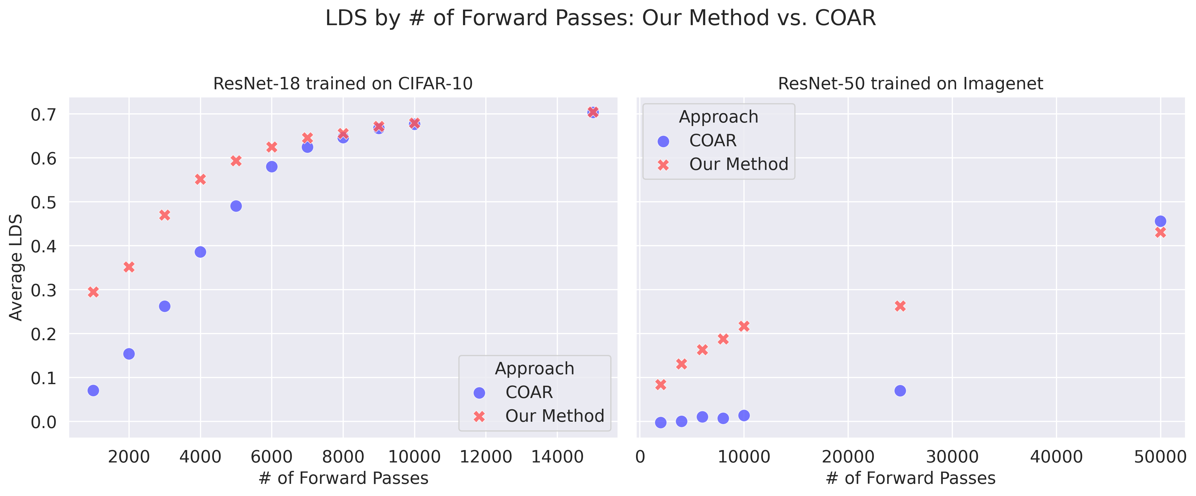
I stumbled upojn a new approach for computing component attribution through linear modeling. Some empirical studies demonstrate that this new method significantly reduces sample complexity while maintaining comparable predictive accuracy benchmarks across various test points z.
For instance, when considering a ResNet-18 model trained on CIFAR-10 and evaluating random test inputs z from the CIFAR-10 test set, our method decreases the required number of ablated forward passes by approximately 40%, 50%, and 60% for achieving LDS scores of 0.5, 0.4, and 0.3 respectively.
On a larger scale, considering a ResNet-50 model trained on ImageNet, our approach achieves a substantial reduction in the necessary ablated forward passes. Specifically, targeting an LDS of 0.1, our method requires approximately 1,000 forward passes compared to the 25,000 needed by COAR—a reduction exceeding 95%.

The Method
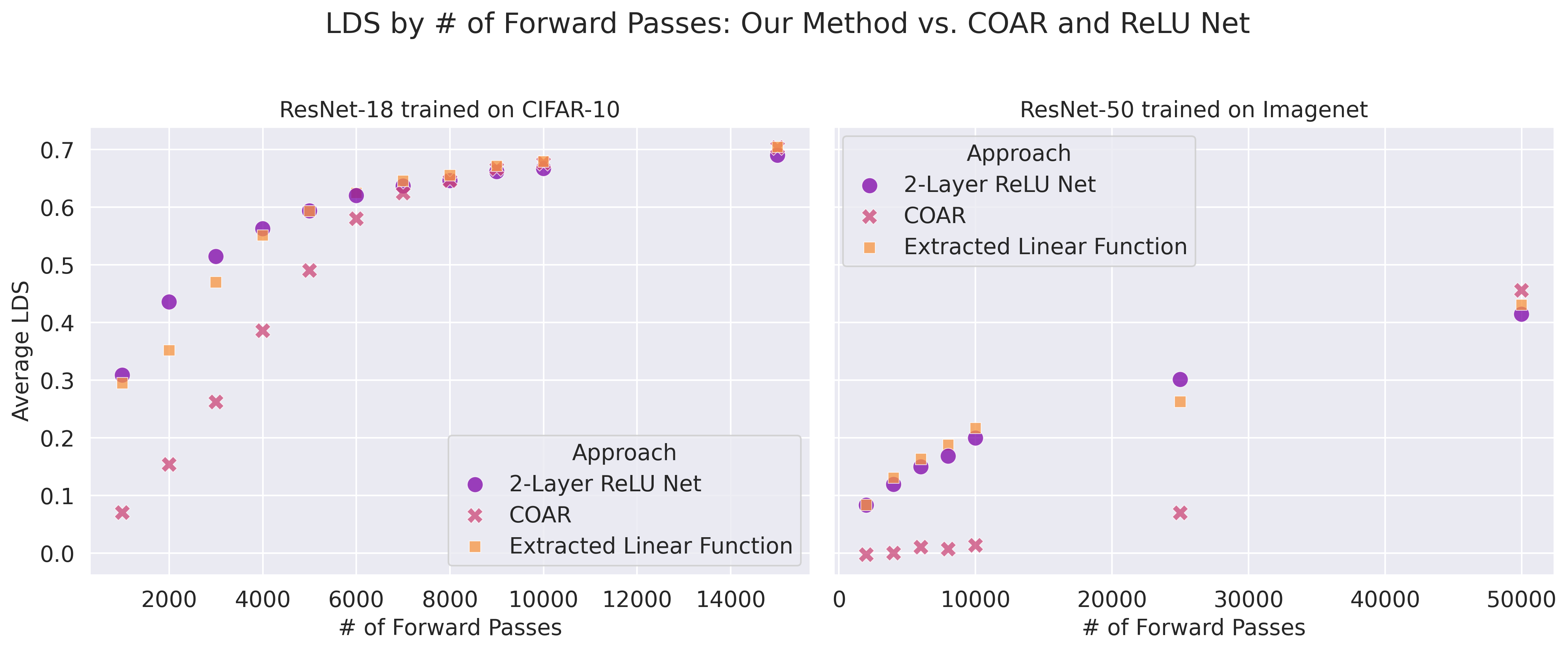
The method follows a similar data generation process as the COAR approach but uses a different training mechanism. We generate a dataset Dz = [x(i), f(Mz(x(i)))]i ∈ m in the manner suggested by COAR. However, instead of relying solely on linear regression, we train a 2-layer ReLU network on this dataset. Although the network is non-linear, we extract a linear function by removing all ReLU activations and directly utilizing the weight matrices.
Formally, consider a 2-layer ReLU network φ: ℝn → ℝ defined as:
$$\phi(x) = W^{(2)} \sigma(W^{(1)}x + b^{(1)}) + b^{(2)}$$
In this equation, σ(⋅) represents the element-wise ReLU activation function, W(2) is a 1 × d weight matrix, W(1) is a d × n weight matrix, and b(1), b(2) are the bias terms for the first and second layers, respectively.
The approach involves the following steps, with the initial two steps mirroring those of COAR:
- Construct a dataset of component counterfactuals by sampling a set S of m ablated models, each with n components. Each model is represented by a vector x ∈ {0,1}n, where xi = 0 indicates the ablation of the ith component. These vectors are sampled independently with a mean of μ.
- For any given test input z, perform m forward passes on the model as indicated by the vectors in S. For each ablated model, record the output Mz(x) and compute the correct class margin f(Mz(x)).
- To learn a component model φz for a specific test input z, apply mini-batch stochastic gradient descent to train the parameters of the 2-layer ReLU network using the dataset Dz and the squared loss function ℓ(y, ŷ) = (y - ŷ)2.
-
Derive the resulting linear attribution function θz: ℝn → ℝ by removing the ReLU activations and combining the weight matrices as follows:
$$θ_z(x) = W^{(2)}W^{(1)}x + W^{(2)}b^{(1)} + b^{(2)}$$

References
- Shah, H., et al. (2024). Decomposing and Editing Predictions by Modeling Model Computation.
- Bereska, J., et al. (2024). Mechanistic Interpretability for AI Safety.
- Ilyas, A., et al. (2022). Datamodels: Predicting Predictions from Training Data.